Introduction
Early phase clinical trials typically employ a hypothesis test as their primary analysis, with this test having two possible outcomes: we will either go to the next stage of evaluation (e.g. a large phase III trial), or we will stop development. In a testing framework these decisions correspond with the rejection of the null hypothesis, or the failure to reject it, respectively.
Some authors have suggested that phase II drug trials can extend this approach to allow for a third intermediate outcome, where we pause if we observe data that is not so bad as to warrant an immediate stop, nor so good as to warrant an immediate go. A similar approach is very common in pilot trials of complex interventions. In both settings, the mechanics are the same: we compute an estimate of the parameter of interest, , and compare it against two thresholds, and , such that
The tout package lets us determine optimal values for
the decision thresholds
and
and the sample size
.
In particular, it will find the smallest possible trial which will
satisfy constraints on the following three operating
characteristics:
- , the probability of proceeding to the main trial when ;
- , the probability of not proceeding to the main trial when ; and
- , the probability of making an immediate stop or go decision when .
A simple example
Suppose the parameter of interest, , is the probability of adherence in the intervention arm of a pilot trial. Suppose further that our null and alternative hypotheses are and , respectively. Using typical type I and II error constraints, and , we can find the smallest design that will ensure a probability of at least that we will obtain a pause decision if the true parameter value is midway between the null and alternative hypotheses:
design <- tout_design(rho_0 = 0.5, rho_1 = 0.7, alpha_nom = 0.05, beta_nom  = 0.2, gamma_nom = 0.5)

design
#> Three-outcome design
#>
#> Sample size: 66
#> Decision thresholds: 38 44
#>
#> alpha = 0.04488955
#> beta = 0.1703036
#> gamma = 0.496394
#>
#> Hypotheses: 0.5 (null), 0.7 (alternative)
#> Modification effect range: 0 0
#> Error probability following an intermediate result: 0.5 0.5
We can visualise the sampling distribution of the test statistic under each hypothesis, highlighting the decisions which will be made:
plot(design)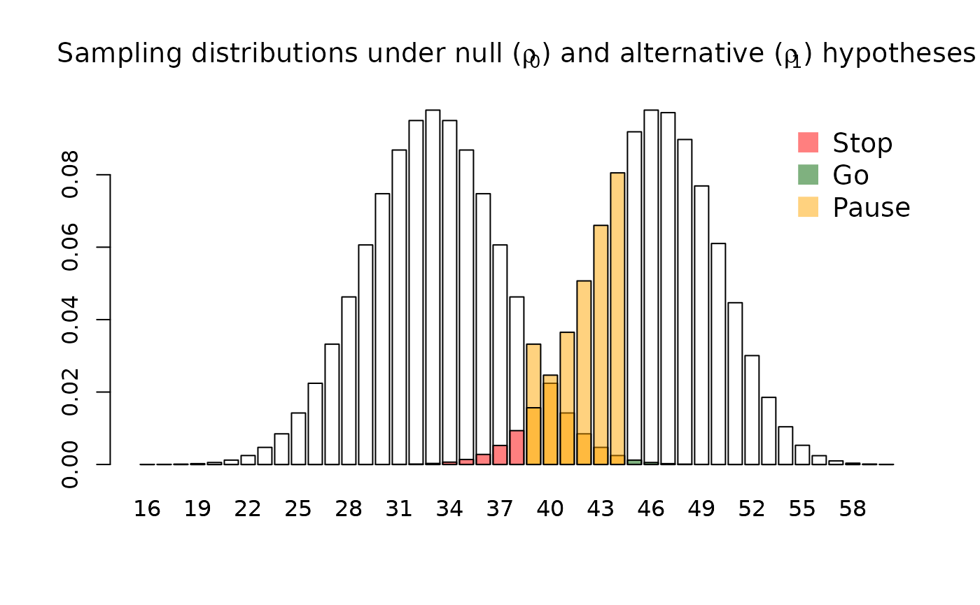
Making decisions following a pause outcome
The testing framework employed in tout acknowledges that
a final stop/go decision must be made following a pause outcome, and
factors this into the calculation of error rates. This requires an
assumption about how well such decisions will be made; in particular, we
must estimate the probabilities that we will incorrectly go when
(denoted
),
and that we will incorrectly stop when
(denoted
).
By default, tout_design() assumes that
,
but we can change these if we wish:
design <- tout_design(rho_0 = 0.5, rho_1 = 0.7, alpha_nom = 0.05, beta_nom  = 0.2, gamma_nom = 0.5, eta_0 = 0.3, eta_1 = 0.4)

design
#> Three-outcome design
#>
#> Sample size: 46
#> Decision thresholds: 26 31
#>
#> alpha = 0.0492724
#> beta = 0.1830351
#> gamma = 0.4863821
#>
#> Hypotheses: 0.5 (null), 0.7 (alternative)
#> Modification effect range: 0 0
#> Error probability following an intermediate result: 0.3 0.4
Making adjustments following a pause outcome
We often anticipate making some adjustments to the intervention
and/or the trial design following a pause outcome, in an attempt to
improve the parameter of interest and ensure the subsequent trial is
successful. We can incorporate this in tout if we can
specify an interval for the effect of this modification
.
For example, suppose we anticipate an improvement in adherence in the
range of
.
The optimal design is then
design <- tout_design(rho_0 = 0.5, rho_1 = 0.7, alpha_nom = 0.05, beta_nom  = 0.2, gamma_nom = 0.5, tau = c(0.01, 0.05))

design
#> Three-outcome design
#>
#> Sample size: 100
#> Decision thresholds: 55 63
#>
#> alpha = 0.04924659
#> beta = 0.1988391
#> gamma = 0.4732802
#>
#> Hypotheses: 0.5 (null), 0.7 (alternative)
#> Modification effect range: 0.01 0.05
#> Error probability following an intermediate result: 0.5 0.5
Designs for continuous endpoints
By default, tout_design() assumes a binary endpoint. We
can find designs for continuous endpoints if we supply the (assumed
known) standard deviation of the outcome via the sigma
argument. For example,
design <- tout_design(rho_0 = 2, rho_1 = 5, alpha_nom = 0.05, beta_nom  = 0.2, gamma_nom = 0.5, sigma = 7, tau = c(1, 2), max_n = 500)

design
#> Three-outcome design
#>
#> Sample size: 179
#> Decision thresholds: -0.6286741 1.644913
#>
#> alpha = 0.05
#> beta = 0.2002572
#> gamma = 0.3147751
#>
#> Hypotheses: 2 (null), 5 (alternative)
#> Standard deviation: 7
#> Modification effect range: 1 2
#> Error probability following an intermediate result: 0.5 0.5
Note that the decision thresholds are given on the scale of the z-statistic.
Further details
For the case of a binary endpoint, the three error rates are formally defined as:
Derivations of these are given in the associated manuscript. The case of continuous endpoints follows, now considering the test statistic to be a z-statistic with distribution
Given any
and
,
the
corresponding to the nominal constraint on
can be found exactly. The optimal
is determined numerically (using an exhaustive search in the binary case
and optimize() in the continuous case) with respect to the
nominal constraint on
.
Finally, a bisection search is used to find the lowest
which satisfies the nominal constraint on
.
References
- Wilson, D.T., Hudson, E. & Brown, S. Three-outcome designs for external pilot trials with progression criteria. BMC Med Res Methodol 24, 226 (2024). https://doi.org/10.1186/s12874-024-02351-x