Examples
Examples.RmdIn this vignette we provide a few example applications of BOSSS.
NIFTy
The NIFTy trial was open to people having total thyroid surgery and aimed to find out whether using near-infrared fluorescence imaging could reduce the number of people whose parathyroid glands become damaged during thyroid surgery. It was an adaptive design with an interim analysis based on a (binary) short-term outcome, and a final analysis based on a (again, binary) long-term outcome.
The design problem here is to choose the sample size and the decision rule for both the inerim and final analysis. Both analyses used a test, so the decision rule could be expressed as the nominal used at each stage.
This is the simulation function, exactly as provided by the trial statistician except for small adjustments to the arguments and return values to conform to the BOSSS standards.
#n is the total sample size
#ninterim is the number of patients at the interim analysis (proportion)
#ainterim is alpha at interim analysis (threshold p-value at interim analysis)
#afinal is alpha at final analaysis (threshold p-value for 2nd and final analysis)
#this means overall alpha for the trial is ainterim*afinal
#
#pcontshort is the probability of 1 day PoSH in the control arm
#pexpshort is the probability of 1 day PoSH in the experimental arm
#pcontlong is the probability of 6 month PoSH in the control arm
#pexplong is the probability of 6 month PoSH in the experimental arm
#p01_relative is s.t. p01_relative*pexplong = probability of having
# a long term outcome after no short term outcome

sim_trial <- function(n = 300, ninterim = 0.5, ainterim = 0.4, afinal = 0.1,
                      pcontshort = 0.25, pexpshort = 0.125,
                      pcontlong = 0.1, pexplong = 0.03, p01_relative = 0)
{
  ninterim <- floor(ninterim*n)

  patients<-c(1:n) #create patients

  treat<- rep(c(1,2), ceiling(n/2))[1:n]

  n_cont <- sum(treat == 1)

  short<-rep(0,n) #short term outcome
  long<-rep(0,n) #long term outcome

  data<-data.frame(patients,treat,short,long) #combine into dataset

  #generate result 1/0 for short term outcome. If short term outcome=0 then long term outcome=0
  #If short term outcome=1 then long term outcome has probability pcontlong/pcontshort
  #repeat for treatment=2
  # for(i in 1:n){
  #   if(treat[i]==1){
  #     data$short[i]<-rbinom(1,1,pcontshort)
  #     if(data$short[i]==0){
  #       data$long[i]<-0
  #     }
  #     if(data$short[i]==1){
  #       data$long[i]<-rbinom(1,1,pcontlong/pcontshort)
  #     }
  #   }
  #   else{
  #     data$short[i]<-rbinom(1,1,pexpshort)
  #     if(data$short[i]==0){
  #       data$long[i]<-0
  #     }
  #     if(data$short[i]==1){
  #       data$long[i]<-rbinom(1,1,pexplong/pexpshort)
  #     }
  #   }
  # }

  # An alternative and more general parametersation of the above model
  # to allow different values of probability of a long outcome after
  # no short outcome (previously hard coded as 0)

  # probability vector p00, p01, p10, p11 in (short, long) form
  # Control arm:
  p01 <- p01_relative*pcontlong
  p11 <- pcontlong - p01
  p10 <- pcontshort - p11
  # Simulate outcomes in multinomial format
  cont_count <- rmultinom(1, n_cont, c((1 - p01 - p10 - p11), p01, p10, p11))
  # Translate these to short and long outcomes
  cont_out <- matrix(c(rep(c(0,0), cont_count[1]),
                       rep(c(0,1), cont_count[2]),
                       rep(c(1,0), cont_count[3]),
                       rep(c(1,1), cont_count[4])), ncol = 2, byrow = TRUE)
  # shuffle the list randomly
  cont_out <- cont_out[sample(1:nrow(cont_out)),]

  # Experimental arm:
    # Control arm:
  p01 <- p01_relative*pexplong
  p11 <- pexplong - p01
  p10 <- pexpshort - p11
  exp_count <- rmultinom(1, n - n_cont, c((1 - p01 - p10 - p11), p01, p10, p11))
  exp_out <- matrix(c(rep(c(0,0), exp_count[1]),
                       rep(c(0,1), exp_count[2]),
                       rep(c(1,0), exp_count[3]),
                       rep(c(1,1), exp_count[4])), ncol = 2, byrow = TRUE)
  exp_out <- exp_out[sample(1:nrow(exp_out)),]

  data[data$treat == 1, c("short", "long")] <- cont_out
  data[data$treat == 2, c("short", "long")] <- exp_out

  #perform chi squared test on short term outcome for 1st ninterim patients
  data2<-data[1:ninterim,]
  tbl<-table(data2$short,data2$treat)
  test<- suppressWarnings(chisq.test(tbl)$p.value) #get p-value

  #if p<ainterim, perform chi squared test on long term outcome for all patients
  if(test<ainterim){
    tbl2<-table(data$long,data$treat)
    test2<- suppressWarnings(chisq.test(tbl2)$p.value)
  }

  #if p>ainterim, trial unsuccessful at interim and final analysis
  #if p<ainterim, trial successful at interim:
  #if p2>afinal, trial unsuccessful at final analysis
  #if p2<afinal, trial successful at final analysis
  if(test>=ainterim){
    return(c(g = FALSE, s = TRUE, n = ninterim))
  }
  if(test<ainterim){
    if(mean(data2[data2$treat == 1,"short"]) < mean(data2[data2$treat == 2,"short"])){
      return(c(g = FALSE, s = TRUE, n = ninterim))
    } else {
      if(test2>afinal){
        return(c(g = FALSE, s = TRUE, n = n))
      }
      if(test2<afinal){
        return(c(g = TRUE, s = FALSE, n = n))
      }
    }
  }
}

# For example,
sim_trial()
We can construct the BOSSS problem object as follows:
# Problem specification
design_space <- design_space(lower = c(300,0.05,0,0),
                             upper = c(700,0.5,1,1),
                             sim = sim_trial)

hypotheses <- hypotheses(values = matrix(c(0.25, 0.25, 0.1, 0.1, 0,
                                           0.25, 0.125, 0.1, 0.03, 0), ncol = 2),
                         hyp_names = c("null", "alt"),
                         sim = sim_trial)

constraints <- constraints(name = c("TI_con", "TII_con"),
                   out = c("g", "s"),
                   hyp = c("null", "alt"),
                   nom = c(0.1, 0.2),
                   delta =c(0.95, 0.95),
                   binary = c(TRUE, TRUE))

objectives <- objectives(name = c("TI", "TII", "EN"),
                 out = c("g", "s", "n"),
                 hyp = c("null", "alt", "null"),
                 weight = c(100, 100, 1),
                 binary = c(TRUE, TRUE, FALSE))

prob <- BOSSS_problem(sim_trial, design_space, hypotheses, objectives, constraints)
This implies we are going to search over a space of sample sizes and
decision criteria, looking for trial designs which simultaneously
minimise the type I error rate ("TI"), type II error rate
("TII") and expected sample size ("EN"),
subject to the type I error rate being (probably) less than 0.1
("TI_con") and the type II error rate being (probably) less
than 0.2 ("TIIcon").
Now we initialise to get an initial estimate of the Pareto front:
set.seed(987953021)

# Initialisation
size <- 40
N <- 500

ptm <- proc.time()
sol <- BOSSS_solution(size, N, prob)
proc.time() - ptm
print(sol)
#> Design variables for the Pareto set:
#>
#>         n  ninterim ainterim   afinal
#> 2  600.00 0.1625000 0.750000 0.250000
#> 9  575.00 0.4156250 0.812500 0.187500
#> 13 625.00 0.3593750 0.437500 0.062500
#> 15 325.00 0.4718750 0.687500 0.312500
#> 22 587.50 0.2046875 0.718750 0.031250
#> 27 462.50 0.4578125 0.781250 0.093750
#> 35 418.75 0.2820313 0.859375 0.328125
#> 37 668.75 0.3382812 0.734375 0.203125
#> 39 368.75 0.4507813 0.484375 0.453125
#>
#> Corresponding objective function values...
#>
#>    g, null (mean) g, null (var) s, alt (mean) s, alt (var) n, null (mean)
#> 2       -2.895870    0.04030898     -1.626804   0.01456830       245.8880
#> 9       -2.581421    0.03058315     -3.463266   0.06790476       362.6900
#> 13      -4.378391    0.16344445     -1.898346   0.01764933       297.7840
#> 15      -2.856301    0.03890908     -1.671131   0.01501243       197.0320
#> 22      -4.556303    0.19448254     -1.461425   0.01308801       269.6000
#> 27      -4.094751    0.12408210     -2.150157   0.02140535       284.9410
#> 35      -2.309640    0.02434019     -2.334207   0.02483631       225.6685
#> 37      -2.856301    0.03890908     -3.276937   0.05706450       349.0845
#> 39      -2.359280    0.02535564     -1.863526   0.01720311       207.7665
#>    n, null (var)
#> 2      105.65737
#> 9       53.05197
#> 13      48.38338
#> 15      11.29196
#> 22      95.30629
#> 27      26.31040
#> 35      41.66091
#> 37      78.84944
#> 39      13.47438
#>
#> ...and constraint function values:
#>
#>    g, null (mean) g, null (var) s, alt (mean) s, alt (var)
#> 2       -2.895870    0.04030898     -1.626804   0.01456830
#> 9       -2.581421    0.03058315     -3.463266   0.06790476
#> 13      -4.378391    0.16344445     -1.898346   0.01764933
#> 15      -2.856301    0.03890908     -1.671131   0.01501243
#> 22      -4.556303    0.19448254     -1.461425   0.01308801
#> 27      -4.094751    0.12408210     -2.150157   0.02140535
#> 35      -2.309640    0.02434019     -2.334207   0.02483631
#> 37      -2.856301    0.03890908     -3.276937   0.05706450
#> 39      -2.359280    0.02535564     -1.863526   0.01720311
plot(sol)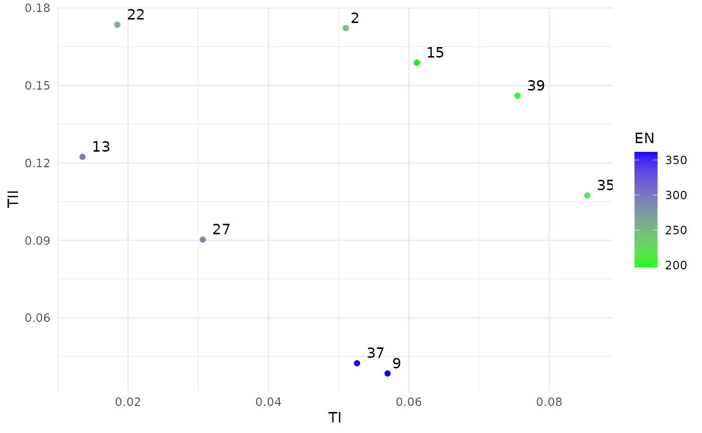
Finally, we iterate a few times to improve that initial approximation:
# Iterations
ptm <- proc.time()
N <- 500
for(i in 1:20) {
  sol <- iterate(sol, prob, N)
}
proc.time() - ptm
print(sol)
#> Design variables for the Pareto set:
#>
#>           n  ninterim   ainterim     afinal
#> 9  575.0000 0.4156250 0.81250000 0.18750000
#> 13 625.0000 0.3593750 0.43750000 0.06250000
#> 15 325.0000 0.4718750 0.68750000 0.31250000
#> 27 462.5000 0.4578125 0.78125000 0.09375000
#> 37 668.7500 0.3382812 0.73437500 0.20312500
#> 39 368.7500 0.4507813 0.48437500 0.45312500
#> 42 693.5662 0.4949120 0.27456863 0.02329762
#> 43 698.4236 0.4747349 0.72489771 0.12223652
#> 45 691.9437 0.4645113 0.73323696 0.27106134
#> 46 450.3917 0.3152930 0.66498311 0.12892175
#> 47 469.9705 0.3903419 0.72850417 0.28434527
#> 48 392.7671 0.2651745 0.71856545 0.29197172
#> 49 437.7276 0.3502485 0.69773093 0.26460208
#> 51 546.2313 0.4977586 0.41949884 0.20778485
#> 53 699.0088 0.4991350 0.33036663 0.11854772
#> 54 348.5348 0.3229493 0.71953816 0.33433016
#> 55 699.3476 0.4948859 0.05700285 0.09839968
#> 56 698.5863 0.4972386 0.20772586 0.08912535
#> 57 698.6434 0.2916672 0.31607825 0.10865194
#> 58 504.1285 0.4338548 0.66805138 0.32772313
#> 59 462.4255 0.2831918 0.58560022 0.14097364
#> 60 691.7141 0.4942135 0.49990569 0.13285708
#>
#> Corresponding objective function values...
#>
#>    g, null (mean) g, null (var) s, alt (mean) s, alt (var) n, null (mean)
#> 9       -2.581421    0.03058315     -3.463266   0.06790476       362.6900
#> 13      -4.378391    0.16344445     -1.898346   0.01764933       297.7840
#> 15      -2.856301    0.03890908     -1.671131   0.01501243       197.0320
#> 27      -4.094751    0.12408210     -2.150157   0.02140535       284.9410
#> 37      -2.856301    0.03890908     -3.276937   0.05706450       349.0845
#> 39      -2.359280    0.02535564     -1.863526   0.01720311       207.7665
#> 42      -7.824446    5.00600080     -2.047467   0.01975463       387.1713
#> 43      -3.276937    0.05706450     -3.397487   0.06384469       447.1059
#> 45      -2.745316    0.03526753     -4.226834   0.14102920       436.7344
#> 46      -3.689289    0.08408277     -1.716844   0.01549312       216.6308
#> 47      -2.437794    0.02707023     -2.521850   0.02906385       270.8130
#> 48      -2.644208    0.03228670     -1.641433   0.01471253       185.4323
#> 49      -2.936892    0.04182035     -1.898346   0.01764933       222.4735
#> 51      -3.335521    0.06025724     -2.411048   0.02647070       329.3490
#> 53      -3.689289    0.08408277     -3.335521   0.06025724       392.2271
#> 54      -2.411048    0.02647070     -1.656207   0.01486053       176.8105
#> 55      -6.030685    0.83600481     -1.583759   0.01415688       355.8937
#> 56      -4.378391    0.16344445     -2.493162   0.02836425       376.5333
#> 57      -4.771895    0.24030264     -1.780150   0.01619872       269.4162
#> 58      -2.285558    0.02386577     -3.118117   0.04929603       300.9773
#> 59      -3.533378    0.07253729     -1.569679   0.01402643       215.7658
#> 60      -3.608458    0.07787237     -3.335521   0.06025724       410.4414
#>    n, null (var)
#> 9      53.051972
#> 13     48.383377
#> 15     11.291958
#> 27     26.310401
#> 37     78.849435
#> 39     13.474383
#> 42     27.121986
#> 43     58.475890
#> 45     59.191370
#> 46     34.961456
#> 47     35.047317
#> 48     33.835167
#> 49     29.968867
#> 51     25.360469
#> 53     27.190516
#> 54     22.303688
#> 55      6.809701
#> 56     19.060671
#> 57     57.129542
#> 58     33.781442
#> 59     42.394723
#> 60     39.142223
#>
#> ...and constraint function values:
#>
#>    g, null (mean) g, null (var) s, alt (mean) s, alt (var)
#> 9       -2.581421    0.03058315     -3.463266   0.06790476
#> 13      -4.378391    0.16344445     -1.898346   0.01764933
#> 15      -2.856301    0.03890908     -1.671131   0.01501243
#> 27      -4.094751    0.12408210     -2.150157   0.02140535
#> 37      -2.856301    0.03890908     -3.276937   0.05706450
#> 39      -2.359280    0.02535564     -1.863526   0.01720311
#> 42      -7.824446    5.00600080     -2.047467   0.01975463
#> 43      -3.276937    0.05706450     -3.397487   0.06384469
#> 45      -2.745316    0.03526753     -4.226834   0.14102920
#> 46      -3.689289    0.08408277     -1.716844   0.01549312
#> 47      -2.437794    0.02707023     -2.521850   0.02906385
#> 48      -2.644208    0.03228670     -1.641433   0.01471253
#> 49      -2.936892    0.04182035     -1.898346   0.01764933
#> 51      -3.335521    0.06025724     -2.411048   0.02647070
#> 53      -3.689289    0.08408277     -3.335521   0.06025724
#> 54      -2.411048    0.02647070     -1.656207   0.01486053
#> 55      -6.030685    0.83600481     -1.583759   0.01415688
#> 56      -4.378391    0.16344445     -2.493162   0.02836425
#> 57      -4.771895    0.24030264     -1.780150   0.01619872
#> 58      -2.285558    0.02386577     -3.118117   0.04929603
#> 59      -3.533378    0.07253729     -1.569679   0.01402643
#> 60      -3.608458    0.07787237     -3.335521   0.06025724

p <- PS_empirical_ests(sol, prob)[[1]][, c(1,3,5)]
p[,1] <- 1/(1 + exp(-p[,1]))
p[,2] <- 1/(1 + exp(-p[,2]))

df <- cbind(sol$p_set[,1:4], p)

df <- df[order(df[,1]),]

colnames(df) <- c("$n$", "$n_{int}$", "$\\alpha_{int}$", "$\\alpha_{f}$",
                       "$E[g ~|~ H_0]$", "$E[s ~|~ H_1]$", "$E[N ~|~ H_0]$")

#print(xtable(df, digits = c(0,0,2,2,2,2,2,0)), booktabs = T, include.rownames = T, sanitize.text.function = function(x) {x}, floating = F, file = here("man", "tables", "NIFTy.txt"))

plot(sol)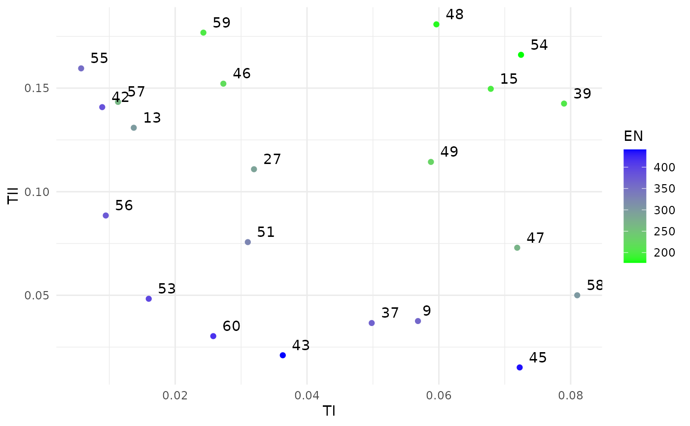
#ggsave(here("man", "figures", "NIFTy.pdf"), height=9, width=14, units="cm")From this set of efficient solutions, suppose we judge number 49 to offer the best trade-offs. Checking that design gives:
design <- sol$p_set[row.names(sol$p_set) == 49,]

r <- diag_check_point(design, prob, sol, N=10^5)

# Model 1 prediction interval: [0.052, 0.066]
# Model 1 empirical interval: [0.06, 0.063]

# Model 2 prediction interval: [0.101, 0.13]
# Model 2 empirical interval: [0.109, 0.113]

# Model 3 prediction interval: [224.613, 233.95]
# Model 3 empirical interval: [230.007, 231.58]
This confirms that this specific design is well within our two constraints, and also suggests the three GP models are fitting the simulated data well.
PRESSURE 2
PRESSURE 2 was a trial comparing different mattresses in terms of their ability to prevent the development of pressure ulcers, with longitudinal data collected on each patient. Smith et al. (2021) suggested one way to analyse this data is through a multi-state model, and showed how simulation could be used to estimate the power of such an analysis. Herw we will extend this approach to searching for an optimal design.
The simulation and deterministic functions are:
sim_P2 <- function(n = 500, fu = 60, af = 1,
                   q12 = 0.05, q23 = 0.05, q34 = 0.03,
                   b12 = 0.67, b23 = 0.67, b34 = 0.67){

  # n: total number of patients
  # fu: follow-up length (days)
  # af: assemment frequency (days)
  # q12, q23, q34: transition probabilities
  # b12, b23, b34: treatment effects

  # Calculate length of follow up
  na <- n*floor(fu/af)

  # Assessment times
  as_times <- floor(seq(af, fu, af))

  # Simulate numbers starting in each state
  starts <- rep(1:3, times = rmultinom(1, n, c(0.15, 0.7, 0.15)))
  # Randomly allocate treatment
  trt <- rbinom(n, 1, 0.5)

  # Simulate transitions into each remaining state
  enter2 <- (starts == 1)*rexp(n, q12*exp(log(b12)*trt))
  enter3 <- (starts != 3)*(enter2 + rexp(n, q23*exp(log(b23)*trt)))
  enter4 <- (starts != 3)*enter3 + rexp(n, q34*exp(log(b34)*trt))

  # Matrix of transition times into each state for each patient
  enter_m <- matrix(c(enter2, enter3, enter4), ncol = 3)

  # Add time of "transitioning" to the end of the follow-up period
  enter_m <- cbind(enter_m, pmax(enter_m[,3], fu))
  # Cap all times at length of follow-up
  enter_m <- pmin(enter_m, fu)

  # Ceiling all times, assuming assessment is at the start of the day
  # and so any transitions after x.0 will be seen at (x+1).0
  enter_m <- ceiling(enter_m)

  # Translate into number of days spent in each state
  times_m <- cbind(enter_m[,1],
                   enter_m[,2] - enter_m[,1],
                   enter_m[,3] - enter_m[,2],
                   enter_m[,4] - enter_m[,3])

  y <- t(apply(times_m, 1, function(x) rep(1:4, times = x)))

  # Reshape to long
  y <- melt(y)
  colnames(y) <- c("id", "time", "state")
  y$trt <- trt[y$id]

  # Keep observations on assessment times and order by patient
  y <- y[y$time %in% as_times,]
  y <- y[order(y$id),]

  Q <- rbind ( c(0, 0.1, 0, 0),
               c(0, 0, 0.1, 0),
               c(0, 0, 0, 0.1),
               c(0, 0, 0, 0) )

  # If msm returns an error we take this as a non-significant result
  suppressWarnings(fit <- try({
    msm(state ~ time, subject=id, data = y, qmatrix = Q,
             covariates = ~ trt)
  }, silent = TRUE))

  if (class(fit) == "try-error") {
    sig <- 0
  } else {
    # If not converged, will not return CIs
    r1.67 <- hazard.msm(fit, cl = 1 - 0.0167)$trt
    if(ncol(r1.67) != 3){
      sig <- 0
    } else {
      sig1.67 <- sum(!(r1.67[,2] < 1 & r1.67[,3] > 1)) >= 3

      r2.5 <- hazard.msm(fit, cl = 1 - 0.025)$trt
      sig2.5 <- sum(!(r2.5[,2] < 1 & r2.5[,3] > 1)) >= 2

      r5 <- hazard.msm(fit, cl = 1 - 0.05)$trt
      sig5 <- sum(!(r5[,2] < 1 & r5[,3] > 1)) >= 1

      sig <- any(c(sig1.67, sig2.5, sig5))
    }
  }
  return(c(s = !sig))
}

det_P2 <- function(n = 500, fu = 60, af = 1,
                   q12 = 0.05, q23 = 0.05, q34 = 0.03,
                   b12 = 0.67, b23 = 0.67, b34 = 0.67){

  na <- n*floor(fu/af)

  return(c(n = n, a = na, f = fu))
}

sim_P2()
We now construct a problem to encode that we want to search over the total number of patients, total number of assessments and the assessment frequency. We are looking for designs which minimise the numbers of pattens and assessments, whilst constraining the type II error rate to be (probably) less than 0.2 and the follow-up length to be less than 200.
design_space <- design_space(lower = c(50, 10, 1),
                             upper = c(500, 60, 10),
                             sim = sim_P2)

hypotheses <- hypotheses(values = matrix(c(0.05, 0.05, 0.03, 0.67, 0.67, 0.67), ncol = 1),
                         hyp_names = c("alt"),
                         sim = sim_P2)

constraints <- constraints(name = c("a"),
                   out = c("s"),
                   hyp = c("alt"),
                   nom = c(0.2),
                   delta =c(0.95),
                   binary = c(TRUE))

objectives <- objectives(name = c("n", "a", "f"),
                 out = c("n", "a", "f"),
                 hyp = c("alt", "alt", "alt"),
                 weight = c(10, 1, 10),
                 binary = c(FALSE, FALSE, FALSE))

prob <- BOSSS_problem(sim_P2, design_space, hypotheses, objectives, constraints, det_func = det_P2)
set.seed(327324)

size <- 30
N <- 100

ptm <- proc.time()
sol <- BOSSS_solution(size, N, prob)
proc.time() - ptm
print(sol)
#> Design variables for the Pareto set:
#>
#>           n      fu      af
#> 9  359.3750 50.6250 8.31250
#> 13 415.6250 44.3750 4.93750
#> 17 317.1875 58.4375 4.09375
#> 21 485.9375 39.6875 9.71875
#> 25 345.3125 42.8125 1.28125
#> 26 457.8125 30.3125 3.53125
#> 29 401.5625 49.0625 6.90625
#>
#> Corresponding objective function values...
#>
#>    n, alt (mean) a, alt (mean) f, alt (mean)
#> 9       359.3750      2156.250       50.6250
#> 13      415.6250      3325.000       44.3750
#> 17      317.1875      4440.625       58.4375
#> 21      485.9375      1943.750       39.6875
#> 25      345.3125     11395.312       42.8125
#> 26      457.8125      3662.500       30.3125
#> 29      401.5625      2810.938       49.0625
#>
#> ...and constraint function values:
#>
#>    s, alt (mean) s, alt (var)
#> 9      -2.419826    0.1333284
#> 13     -3.131345    0.2494842
#> 17     -3.131345    0.2494842
#> 21     -2.560667    0.1502170
#> 25     -2.907321    0.2036231
#> 26     -3.798549    0.4665877
#> 29     -3.798549    0.4665877
plot(sol)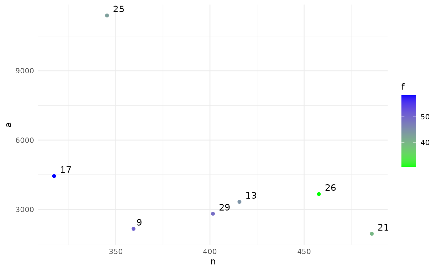
print(sol)
#> Design variables for the Pareto set:
#>
#>           n       fu       af
#> 31 228.5281 49.35014 3.796745
#> 32 436.0485 24.43320 3.054609
#> 33 427.0384 25.46592 2.831004
#> 35 375.1751 35.87907 7.225270
#> 36 299.7509 33.84992 2.426087
#> 37 266.0080 45.64281 5.707002
#> 38 409.0015 39.50040 9.875706
#> 39 460.2070 27.09531 5.422619
#> 40 210.6164 53.24293 3.328948
#> 41 351.2584 29.99896 3.340470
#> 42 460.0331 28.08401 5.657101
#> 43 492.5110 22.98154 2.639792
#> 44 284.9192 51.21357 8.542463
#> 45 224.9842 52.27752 5.274293
#> 46 497.8736 20.94598 2.201160
#> 48 198.2200 56.76570 2.842515
#> 49 257.5549 39.58456 2.950562
#>
#> Corresponding objective function values...
#>
#>    n, alt (mean) a, alt (mean) f, alt (mean)
#> 31      228.5281      2742.337      49.35014
#> 32      436.0485      3052.340      24.43320
#> 33      427.0384      3416.307      25.46592
#> 35      375.1751      1500.700      35.87907
#> 36      299.7509      3896.762      33.84992
#> 37      266.0080      1862.056      45.64281
#> 38      409.0015      1227.004      39.50040
#> 39      460.2070      1840.828      27.09531
#> 40      210.6164      3159.247      53.24293
#> 41      351.2584      2810.067      29.99896
#> 42      460.0331      1840.132      28.08401
#> 43      492.5110      3940.088      22.98154
#> 44      284.9192      1424.596      51.21357
#> 45      224.9842      2024.858      52.27752
#> 46      497.8736      4480.862      20.94598
#> 48      198.2200      3766.181      56.76570
#> 49      257.5549      3348.214      39.58456
#>
#> ...and constraint function values:
#>
#>    s, alt (mean) s, alt (var)
#> 31     -1.442005   0.06465620
#> 32     -1.317975   0.06003526
#> 33     -2.179642   0.10956219
#> 35     -1.648184   0.07389930
#> 36     -1.648184   0.07389930
#> 37     -1.648184   0.07389930
#> 38     -1.648184   0.07389930
#> 39     -1.378841   0.06222167
#> 40     -1.723706   0.07783667
#> 41     -1.442005   0.06465620
#> 42     -1.576338   0.07043940
#> 43     -1.978171   0.09367830
#> 44     -1.978171   0.09367830
#> 45     -1.507734   0.06737895
#> 46     -1.803428   0.08235156
#> 48     -1.648184   0.07389930
#> 49     -1.442005   0.06465620

p <- PS_empirical_ests(sol, prob)[[2]][, 1]
p <- 1 - 1/(1 + exp(-p))

df <- sol$p_set[,1:3]
df$a <- (df$fu %/% df$af)*df$n

df <- cbind(df, p)

df <- df[order(df[,1]),]

colnames(df) <- c("$n$", "$f$", "$a_f$", "a",
                       "$E[s ~|~ H_1]$")

#print(xtable(df, digits = c(0,0,0,0,0,2)), booktabs = T, include.rownames = T, sanitize.text.function = function(x) {x}, floating = F, file = here("man", "tables", "P2.txt"))

plot(sol)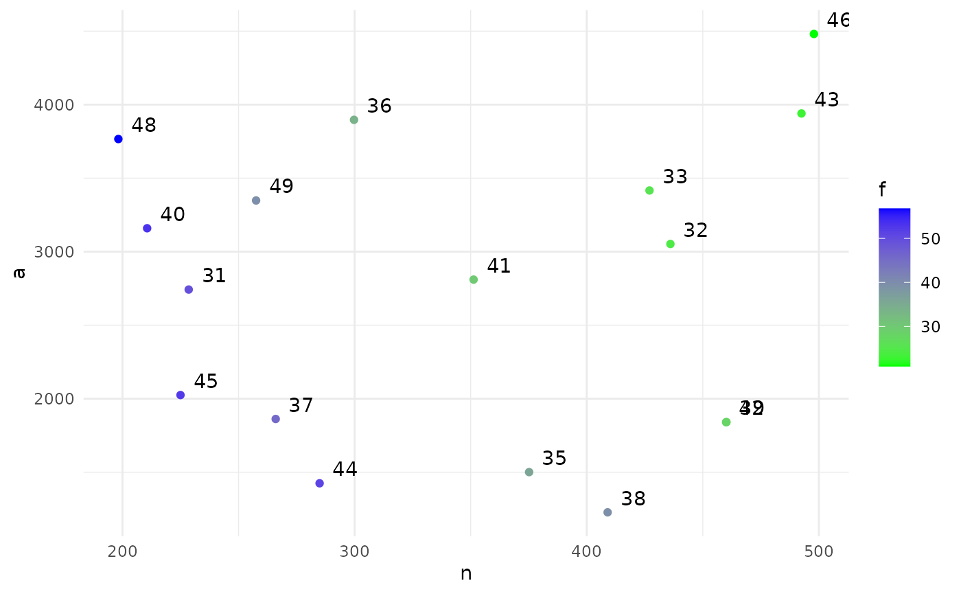
#ggsave(here("man", "figures", "P2.pdf"), height=9, width=14, units="cm")Recruitment
Consider a standard two-arm parallel group trial with a continuous endpoint and a t-test of the group means as the planned analysis. Suppose that we are concerned about how well this trial will recruit, and would like to estimate what the overall probability of a significant result will be when we allow for the uncertainty in attained sample size. We can approach this by using a hierarchical Poisson-Gamma model of multi-site recruitment, with site setup times following a Poisson process. To account for the uncertainty around the true parameter values in that recruitment model we take a Bayesian view and give priors for each parameter. This view then also extends to our outcome model, and we place priors on the mean difference and the outcome standard deviation too.
The design problem here is to choose both the number of recruiting sites and the length of the recruitment period. The model parameters are the hyperparameters of our prior distributions. We want to set a constraint on the unconditional probability of a type II error under the hypothesis of interest, and want to minimise the number of sites and the recruitment period subject to that constraint. We want a simulation function which returns the conditional power (conditioning on the attained sample size and the parameters of the outcome model) for any given design and hypothesis, and a deterministic function to return the two objective functions.
library(BOSSS)

sim_rec <- function(m=20, t=3,
                    a=7, b=2, c=2, d=0.8,
                    f=10, g=1,
                    j=0.3, k=0.3, x=1, y=0.2)
{
  # m - total number of sites to be set up
  # t - time (in years) for recruitment
  # a, b - hyperparameters for rec mean (gamma)
  # c, d - hyperparameters for rec sd (gamma)
  # f, g - hyperparameters for eta (gamma)
  # j, k - hyperparameters for delta (normal)
  # x, y - hyperparameters for sigma (gamma)

  # Sample parameters from their priors
  # Recruitment rate
  alpha <- rgamma(1, (a/b)^2, scale = b^2/a)
  beta <- rgamma(1, (c/d)^2, scale = d^2/c)
  # Setup rate
  eta <- rgamma(1, (f/g)^2, scale = g^2/f)
  # Treatment effect
  delta <- rnorm(1, j, k)
  # Outcome sd
  sigma <- rgamma(1, (x/y)^2, scale = y^2/x)

  # True per year recruitment rates for each site
  lambdas <- rgamma(m, alpha, scale=beta)

  # Setup times
  setup_ts <- cumsum(rexp(m, eta))

  # For each site, simulate number recruited by end
  rec_times <- pmax(t - setup_ts, 0)
  ns <- rpois(m, lambdas*rec_times)

  # Total recruited at final
  end_n <- sum(ns)

  # Cap at target recruitment
  end_n <- min(end_n, 352)

  # Power at analysis
  pow <- power.t.test(n = end_n/2, delta = delta, sd = sigma)$power
  pow

  return(c(pr_tII = 1 - pow))
}

det_rec <- function(m=20, t=3,
                    a=7, b=2, c=2, d=0.8,
                    f=10, g=1,
                    j=0.3, k=0.3, x=1, y=0.2)
{
  return(c(m = floor(m), t = t))
}


# For example,
sim_rec()
Now we set up the problem using the BOSSS helper
functions. We are going to look at designs with between 3 and 40 sites,
running from between 6 months and 5 years.
# Problem specification
design_space <- design_space(lower = c(3,0.5),
                             upper = c(40,5),
                             sim = sim_rec)

hypotheses <- hypotheses(values = matrix(c(7, 2, 2, 0.8,
                                           10, 1, 0.3, 0.3, 1, 0.2), ncol = 1),
                         hyp_names = c("alt"),
                         sim = sim_rec)

constraints <- constraints(name = c("TII_ass"),
                   out = c("pr_tII"),
                   hyp = c("alt"),
                   nom = c(0.4),
                   delta =c(0.95),
                   binary = c(FALSE))

objectives <- objectives(name = c("Sites", "Time"),
                 out = c("m", "t"),
                 hyp = c( "alt", "alt"),
                 weight = c(1, 10),
                 binary = c(FALSE, FALSE))

prob <- BOSSS_problem(sim_rec, design_space, hypotheses, objectives, constraints, det_func = det_rec)
size <- 20
N <- 500

sol <- BOSSS_solution(size, N, prob)

print(sol)
plot(sol)References
Croft J, Ainsworth G, Corrigan N, et al. NIFTy: near-infrared fluorescence (NIRF) imaging to prevent postsurgical hypoparathyroidism (PoSH) after thyroid surgery—a phase II/III pragmatic, multicentre randomised controlled trial protocol in patients undergoing a total or completion thyroidectomy. BMJ Open, 15:e092422 (2025). https://doi.org/10.1136/bmjopen-2024-092422
Nixon, Jane et al. Pressure Relieving Support Surfaces for Pressure Ulcer Prevention (PRESSURE 2): Clinical and Health Economic Results of a Randomised Controlled Trial. eClinicalMedicine, Volume 14, 42 - 52 (2019)
Smith IL, Nixon JE, Sharples L. Power and sample size for multistate model analysis of longitudinal discrete outcomes in disease prevention trials. Statistics in Medicine, 40: 1960–1971 (2021). https://doi.org/10.1002/sim.8882
knitr::knit_exit()