BOSSS

library(BOSSS)
library(ggplot2)
library(mco)

Every application of BOSSS follows the same set of steps:

1. Formally specify the problem and create a corresponding BOSSS_problem object;
2. Create a BOSSS_solution object and initialise it;
3. Perform a number of iterations, each one updating and (hopefully) improving the BOSSS_solution object;
4. Select a final design and run some diagnostics to check it is valid.

We will work through these steps here for an example problem: designing a cluster randomised trial, as discussed in Section 2 of the manuscript associated with the package. For more illustrations, see the article.

Problem

The first ingredient of a BOSSS problem is the simulation function. The arguments of this function must first specify the design variables which we want to vary in our problem, followed by the model parameters. In this example we have two design variables representing the number of clusters in each arm, and the number of participants in each arm. The model parameters are the mean difference in outcome between the control and experimental arms (beta_1), the within-cluster variance (var_e), and the between-cluster variance (var_u). Note that all of these inputs require some defaults to be provided.

The other element of interface the simulation function must conform to is in its return value, which should be a named vector of the quantities who’s mean values we want to estimate using the Monte Carlo method. Here, we have one such quantity: a boolean indicator of a negative decision, s.

sim_cRCT <- function(m = 10, n = 20, 
                     beta_1 = 0.3, var_e = 0.95, var_u = 0.05){
  
  m <- floor(m); n <- floor(n)
  
  x <- rep(c(0,1), each = m) 
  y <- rnorm(2*m, 0, sqrt(var_u + var_e/n))
  y <- y + x*beta_1

  s <- t.test(y[x==1], y[x==0], alternative = "greater")$p.value > 0.025

  return(c(s = s))
}

# For example,
sim_cRCT()
#>     s 
#> FALSE

In our problem we are not just interested in the expected value of s; we also want to minimise the number of clusters and the number of participants. Since these are fixed quantities given any design, we evaluate them in a separate deterministic function. This should conform to the same principles as the simulation function, with the same inputs, but allowing for different named outputs. Here, the outputs are just m, and N = n*m:

det_cRCT <- function(m = 10, n = 5, 
                     beta_1 = 0.3, var_e = 0.95, var_u = 0.05)
{
  return(c(m = floor(m), N = floor(n)*floor(m)))
}  

Next, we need to note the ranges of the design variables which we plan to search over. We use the design_space() function for this, specifying the lower and upper limits of the design variables in the order they appear as simulation function arguments:

design_space <- design_space(lower = c(10, 5), 
                             upper = c(50, 20),
                             sim = sim_cRCT)

design_space
#>   name lower upper
#> 1    m    10    50
#> 2    n     5    20

Note that the function automatically retrieves the names of the design variables based on the order they take in the simulation function.

We also need to specify the hypotheses which we’re planning to simulate under, using the hypotheses() function, again specifying in the order that parameters appear as simulation function argument. We only need one hypothesis here, the alternative, since we will be estimating the type II error rate.

hypotheses <- hypotheses(values = matrix(c(0.3, 0.95, 0.05), ncol = 1),
                         hyp_names = c("alt"),
                         sim = sim_cRCT)

hypotheses
#>         alt
#> beta_1 0.30
#> var_e  0.95
#> var_u  0.05

Constraints should be specified using the constraints function. Each constraint should be named, and should be defined with respect to a specific output and a specific hypothesis. It should have a nominal maximum value, and a probability delta used to judge if it is satisfied. Here, our constraint is that the mean of the simulation output (i.e. the probability of a negative result) under the alt hypothesis should be less than or equal to 0.2 with a probability of at least 0.95. Finally, we note whether the constraint output is binary or otherwise.

constraints <- constraints(name = c("con_tII"),
                   out = c("s"),
                   hyp = c("alt"),
                   nom = c(0.2),
                   delta = c(0.95),
                   binary = c(TRUE))

constraints
#>      name out hyp nom delta binary
#> 1 con_tII   s alt 0.2  0.95   TRUE

The final ingredient of the problem is the set of objectives we want to minimise. Similar to constraints, objectives are tied to a specific output and hypothesis. We also specify weights for each objective which help guide the internal optimisation process, and note whether or not the output for each objective is binary or continuous. For example, here we want to minimise both the number of patients N and the number of clusters m, with the latter carrying a weight of 100 times that of the former.

objectives <- objectives(name = c("N", "m"),
                 out = c("N", "m"),
                 hyp = c("alt", "alt"),
                 weight = c(1, 10),
                 binary = c(FALSE, FALSE))

objectives
#>   name out hyp weight binary
#> 1    N   N alt      1  FALSE
#> 2    m   m alt     10  FALSE

We now put this simulation function and set of data frames together to create an object of class BOSSS_problem.

prob <- BOSSS_problem(sim_cRCT, design_space, hypotheses, objectives, constraints, det_func = det_cRCT)

Initialisation

Having set up the problem, we now need to create an initial solution to it. This involves setting up a space-filling set of designs spanning the design space (where size is the number of designs), computing the Monte Carlo estimates of all the expectations we are interested in at each of these designs (using N samples for each evaluation), fitting Gaussian Process models to these estimates, and then using those models to estimate the Pareto set and front:

set.seed(9823579)

size <- 20
N <- 100

sol <- BOSSS_solution(size, N, prob)
#> Checking simulation speed...
#> Initialisation will take approximately 0.5868146 secs 
#> Solution found

print(sol) 
#> Design variables for the Pareto set: 
#> 
#>        m        n
#> 2  40.00  8.75000
#> 19 23.75 15.78125
#> 
#> Corresponding objective function values...
#> 
#>    N, alt (mean) m, alt (mean)
#> 2            320            40
#> 19           345            23
#> 
#> ...and constraint function values:
#> 
#>    s, alt (mean) s, alt (var)
#> 2      -2.419826    0.1333284
#> 19     -1.442005    0.0646562
plot(sol)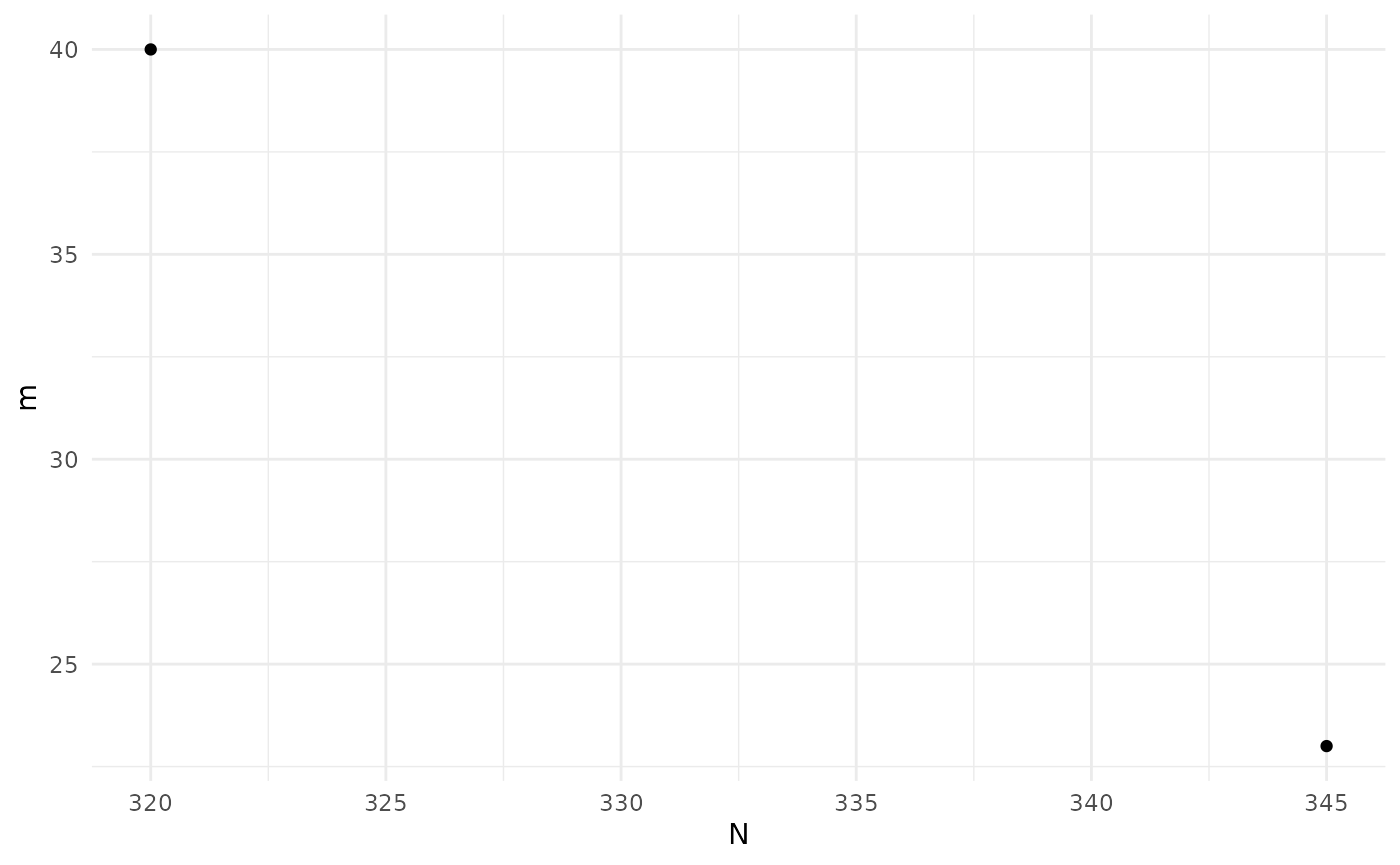

sol_init <- sol

The print() function will give a table of the Pareto set with associated objective function values. The plot() function will plot the Pareto front.

Iteration

We can now start improving this solution by calling the iterate() function. Each call uses the fitted Gaussian Process models to decide on the next design to be evaluated, computes the Monte Carlo estimates at that point, and then updates the estimated Pareto set and front.

N <- 100
for(i in 1:20) {
  sol <- iterate(sol, prob, N) 
}
print(sol)
#> Design variables for the Pareto set: 
#> 
#>           m         n
#> 19 23.75000 15.781250
#> 23 26.99935 11.997542
#> 26 20.99972 19.999855
#> 29 24.97515 13.999811
#> 31 32.99968  8.999911
#> 33 27.95746 10.990021
#> 34 36.93869  7.994242
#> 36 22.97379 16.990697
#> 40 21.99923 17.975259
#> 
#> Corresponding objective function values...
#> 
#>    N, alt (mean) m, alt (mean)
#> 19           345            23
#> 23           286            26
#> 26           380            20
#> 29           312            24
#> 31           256            32
#> 33           270            27
#> 34           252            36
#> 36           352            22
#> 40           357            21
#> 
#> ...and constraint function values:
#> 
#>    s, alt (mean) s, alt (var)
#> 19     -1.442005   0.06465620
#> 23     -1.507734   0.06737895
#> 26     -1.259177   0.05806410
#> 29     -1.648184   0.07389930
#> 31     -1.507734   0.06737895
#> 33     -1.317975   0.06003526
#> 34     -1.202247   0.05628104
#> 36     -1.576338   0.07043940
#> 40     -1.978171   0.09367830
plot(sol)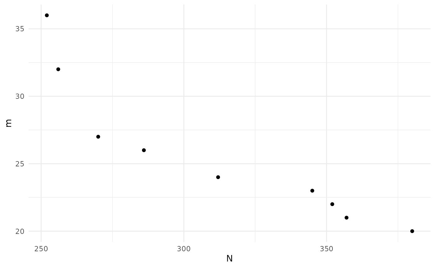

sol_final <- sol

We can compare the initial and final approximations to the Pareto front to the actual front since, for this simple example, we can calculate power analytically:

df <- expand.grid(m = 10:50,
                  n = 5:20)
df$N <- df$m*df$n

df$clust_var <- 0.05 + 0.95/df$n

df$pow <- power.t.test(df$m, delta = 0.3, sd = sqrt(df$clust_var),
                       alternative = "one.sided", sig.level = 0.025)$power

df <- df[df$pow >= 0.8, c("m", "n", "N")]
df <-  data.frame(paretoFilter(as.matrix(df)))
df$t <- "True"

df <- rbind(df, data.frame(m = c(floor(sol_init$p_set$m),
                                 floor(sol_final$p_set$m)),
                           n = c(floor(sol_init$p_set$n),
                                 floor(sol_final$p_set$n)),
                           N = c(floor(sol_init$p_set$N),
                                 floor(sol_final$p_set$N)),
                           t = c(rep("Initial", nrow(sol_init$p_set)),
                                 rep("Final", nrow(sol_final$p_set)))))

# Add ends of steps
df2  <- rbind(data.frame(m=rep(max(df$m), 3),
                          N=c(min(df[df$t == "Initial", "N"]),
                              min(df[df$t == "True", "N"]),
                              min(df[df$t == "Final", "N"])),
                          t=c("Initial", "True", "Final")),
              df[,c("m", "N", "t")],
              data.frame(m=c(min(df[df$t == "Initial", "m"]),
                             min(df[df$t == "True", "m"]),
                             min(df[df$t == "Final", "m"])),
                         N=rep(max(df$N), 3),
                         t=c("Initial", "True", "Final")))

ggplot(df, aes(N, m, colour = t)) + geom_point() +
  xlab("Total sample size per arm, N") +
  ylab("Number of clusters per arm, m") +
  scale_colour_manual(name = "", values = c("#EF476F", "#FFD166", "#06D6A0")) +
  geom_step(data=df2, alpha = 0.5) +
  theme_minimal()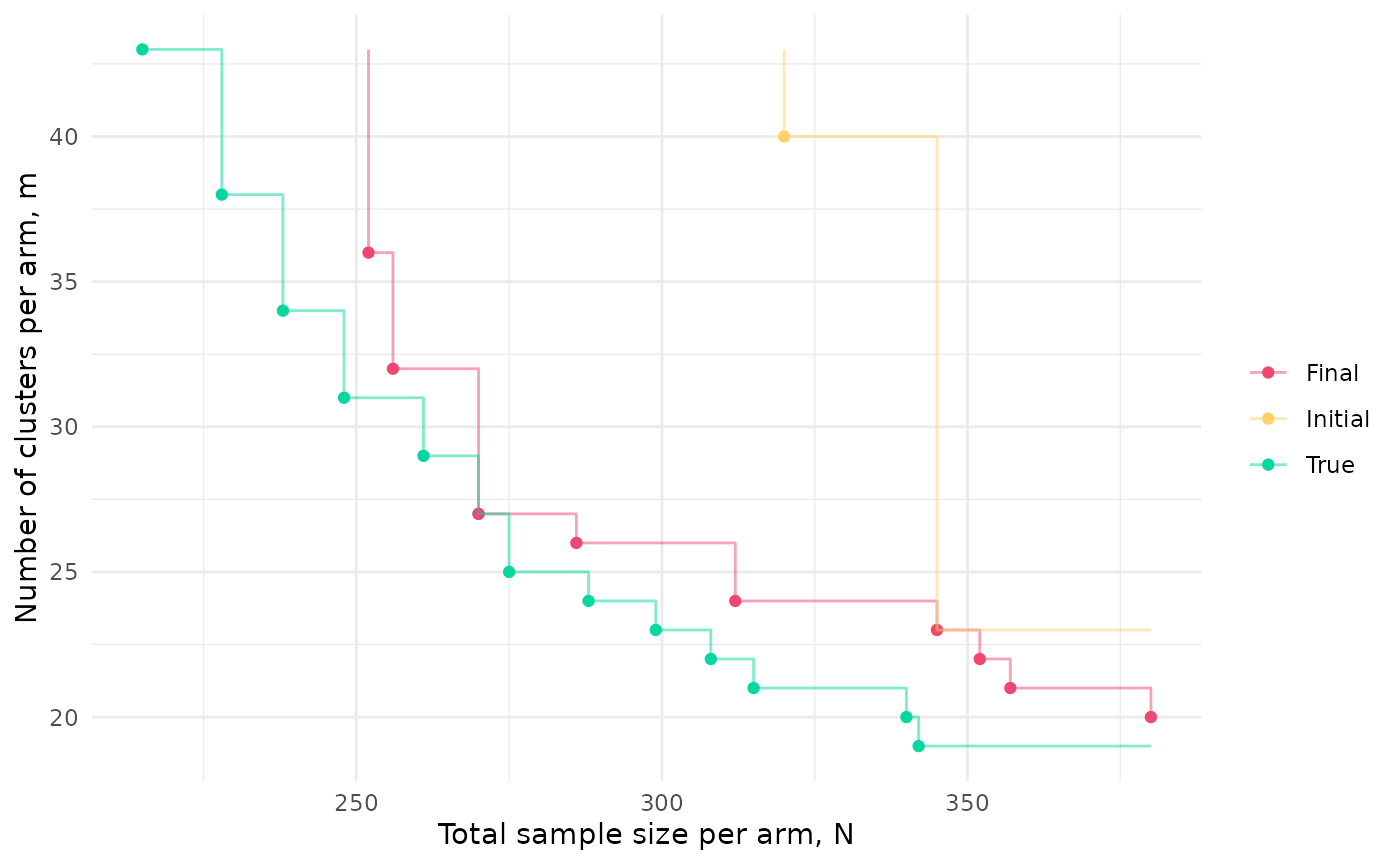

#ggsave(here("man", "figures", "cRCT_fronts.pdf"), height=9, width=14, units="cm")

# Tabulate results
df_init <- df[df$t == "Initial",]
p <- PS_empirical_ests(sol_init, prob)[[2]][,1]
df_init$pow <- 1 - 1/(1 + exp(-p))
df_init <- df_init[order(df_init$m), c(1,2,3,5)]
  
colnames(df_init) <- c("$m$", "$n$", "$N$", "power")

#print(xtable(df_init, digits = c(0,0,0,0,2)), booktabs = T, include.rownames = F, sanitize.text.function = function(x) {x}, floating = F, file = here("man", "tables", "cRCT_init.txt"))

df_final <- df[df$t == "Final",]
p <- PS_empirical_ests(sol_final, prob)[[2]][,1]
df_final$pow <- 1 - 1/(1 + exp(-p))
df_final <- df_final[order(df_final$m), c(1,2,3,5)]
  
colnames(df_final) <- c("$m$", "$n$", "$N$", "power")

#print(xtable(df_final, digits = c(0,0,0,0,2)), booktabs = T, include.rownames = F, sanitize.text.function = function(x) {x}, floating = F, file = here("man", "tables", "cRCT_final.txt"))

Diagnostics

To check the GP models are giving sensible predictions, we can choose a specific design and then plot the predictions for each model along the range of each design variable.

# Pick a specific design from the Pareto set
design <- sol$p_set[1,]

ps <- diag_plots(design, prob, sol)

ps[[1]]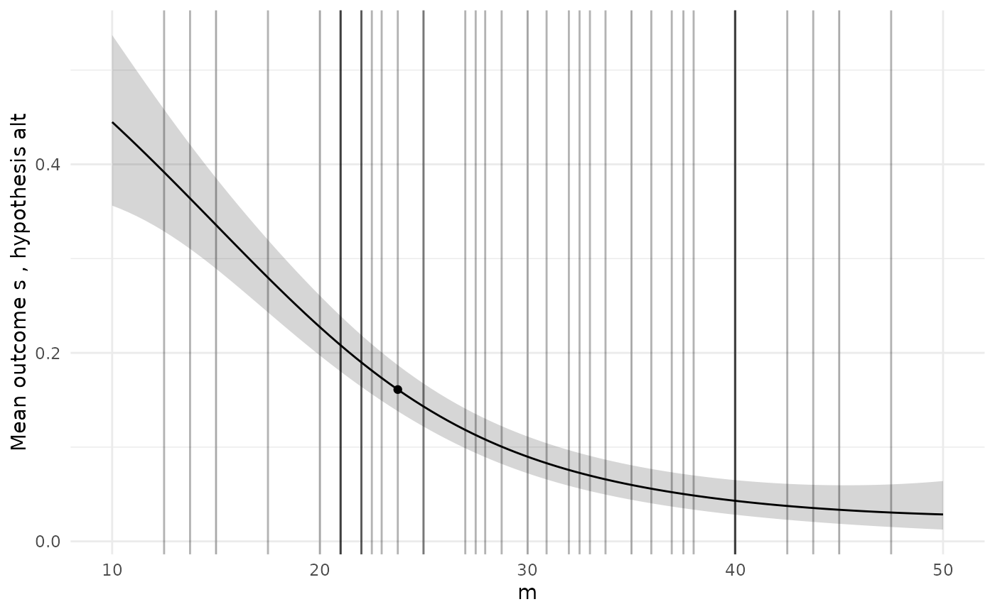

#ggsave(here("man", "figures", "cRCT_diag_m.pdf"), height=8, width=8, units="cm")

ps[[2]]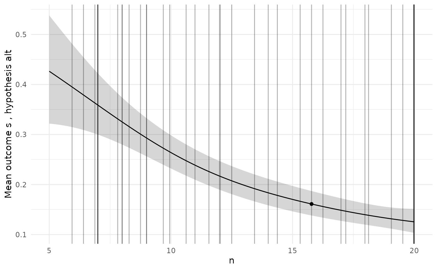

#ggsave(here("man", "figures", "cRCT_diag_n.pdf"), height=8, width=8, units="cm")

We can also get the predicted values and 95% credible intervals for each point we have evaluated, contrasting these with the empirical MC estimate and interval. This will return a data frame for each of the models, named according to the output-hypothesis combination which defines it. We highlight with a * any points where the two intervals do not overlap.

diag_predictions(prob, sol)
#> $`Output: s, hypothesis: alt`
#>           m         n    MC_mean      MC_l95     MC_u95     p_mean      p_l95
#> 1  30.00000 12.500000 0.11155378 0.063118649 0.18963338 0.12762251 0.10772147
#> 2  40.00000  8.750000 0.08167331 0.041666820 0.15392252 0.13890888 0.11684352
#> 3  20.00000 16.250000 0.21115538 0.142069426 0.30201037 0.22166509 0.19147619
#> 4  25.00000 10.625000 0.18127490 0.117482371 0.26914262 0.22750507 0.19918432
#> 5  45.00000 18.125000 0.01195219 0.001988476 0.06841874 0.02556474 0.01226616
#> 6  35.00000  6.875000 0.23107570 0.158794949 0.32360083 0.23138686 0.20070363
#> 7  15.00000 14.375000 0.44023904 0.346374267 0.53858093 0.35342547 0.30492322
#> 8  17.50000  9.687500 0.40039841 0.309210032 0.49905109 0.38829725 0.33317646
#> 9  37.50000 17.187500 0.06175299 0.028329144 0.12936153 0.04308112 0.02818094
#> 10 47.50000  5.937500 0.20119522 0.133803478 0.29112177 0.19624201 0.14331310
#> 11 27.50000 13.437500 0.11155378 0.063118649 0.18963338 0.13983730 0.11872020
#> 12 22.50000  7.812500 0.37051793 0.281742889 0.46900021 0.35198590 0.29843680
#> 13 42.50000 15.312500 0.03187251 0.010672159 0.09130098 0.03995067 0.02444646
#> 14 32.50000 11.562500 0.10159363 0.055809001 0.17786349 0.12213350 0.10254115
#> 15 12.50000 19.062500 0.35059761 0.263632739 0.44876675 0.35459382 0.28675581
#> 16 13.75000 12.031250 0.35059761 0.263632739 0.44876675 0.41355431 0.35217076
#> 17 33.75000 19.531250 0.02191235 0.005838964 0.07872833 0.04749012 0.03065901
#> 18 43.75000  8.281250 0.12151394 0.070564158 0.20128432 0.13509492 0.10727229
#> 19 23.75000 15.781250 0.19123506 0.125606506 0.28016698 0.16106173 0.13743118
#> 20 28.75000  6.406250 0.28087649 0.201616667 0.37659748 0.30993552 0.25660633
#> 21 31.98561  8.998203 0.18127490 0.117482371 0.26914262 0.18663142 0.16437288
#> 22 21.99748 19.995216 0.17131474 0.109435453 0.25804488 0.15091308 0.12657099
#> 23 26.99935 11.997542 0.18127490 0.117482371 0.26914262 0.16935818 0.14637433
#> 24 21.99730 19.976786 0.12151394 0.070564158 0.20128432 0.15103828 0.12678562
#> 25 39.97274  6.988479 0.14143426 0.085811927 0.22426578 0.19393465 0.16840712
#> 26 20.99972 19.999855 0.22111554 0.150400931 0.31283581 0.16720993 0.14127366
#> 27 37.99189  6.993664 0.23107570 0.158794949 0.32360083 0.20584294 0.18005862
#> 28 39.99514  6.998776 0.18127490 0.117482371 0.26914262 0.19344642 0.16798199
#> 29 24.97515 13.999811 0.16135458 0.101470755 0.24686949 0.16480626 0.14107123
#> 30 39.99366  6.999902 0.26095618 0.184326258 0.35555664 0.19341562 0.16795954
#> 31 32.99968  8.999911 0.18127490 0.117482371 0.26914262 0.17763129 0.15617459
#> 32 35.95488  7.996821 0.19123506 0.125606506 0.28016698 0.18555315 0.16397734
#> 33 27.95746 10.990021 0.21115538 0.142069426 0.30201037 0.17805154 0.15493518
#> 34 36.93869  7.994242 0.23107570 0.158794949 0.32360083 0.17893502 0.15774364
#> 35 20.99066 19.995778 0.19123506 0.125606506 0.28016698 0.16739322 0.14146170
#> 36 22.97379 16.990697 0.17131474 0.109435453 0.25804488 0.16039072 0.13758832
#> 37 30.91326  9.949006 0.15139442 0.093594026 0.23561162 0.17071928 0.14900537
#> 38 20.99732 19.985637 0.12151394 0.070564158 0.20128432 0.16735196 0.14148721
#> 39 20.99805 19.995083 0.14143426 0.085811927 0.22426578 0.16727238 0.14135857
#> 40 21.99923 17.975259 0.12151394 0.070564158 0.20128432 0.16681275 0.14450253
#>         p_u95 no_overlap
#> 1  0.15057972           
#> 2  0.16436568           
#> 3  0.25511186           
#> 4  0.25855250           
#> 5  0.05251463           
#> 6  0.26520450           
#> 7  0.40514579           
#> 8  0.44643203           
#> 9  0.06532988           
#> 10 0.26272398           
#> 11 0.16401151           
#> 12 0.40953454           
#> 13 0.06463631           
#> 14 0.14486506           
#> 15 0.42883130           
#> 16 0.47774684           
#> 17 0.07286656           
#> 18 0.16876955           
#> 19 0.18787045           
#> 20 0.36884873           
#> 21 0.21114250           
#> 22 0.17897734           
#> 23 0.19512602           
#> 24 0.17897931           
#> 25 0.22229731           
#> 26 0.19681647           
#> 27 0.23426463           
#> 28 0.22174224           
#> 29 0.19164367           
#> 30 0.22170181           
#> 31 0.20133254           
#> 32 0.20925728           
#> 33 0.20378516           
#> 34 0.20228952           
#> 35 0.19698761           
#> 36 0.18615643           
#> 37 0.19487286           
#> 38 0.19686073           
#> 39 0.19684762           
#> 40 0.19179528

In this example we see that the empirical estimates agree with the predictions for all of the designs which have been evaluated. Once we are happy with our solution and have chosen a specific design from the Pareto set, we might want to double check that point by running a large number of simulations at it:

design <- sol$p_set[1,]
r <- diag_check_point(design, prob, sol, N=10^5) 
#> Model 1 prediction interval: [0.137, 0.188]
#> Model 1 empirical interval: [0.157, 0.161]

At any point, but especially after initialisation, we may decide that we need more points in our initial evaluations, or more simulations at each of the points evaluated so far. We can do that via extend_initial(). For example, suppose we started off with only 10 evaluations at each of 6 initial designs:

set.seed(98579)

size <- 6
N <- 10

sol <- BOSSS_solution(size, N, prob)
#> Checking simulation speed...
#> Initialisation will take approximately 0.01511574 secs 
#> Solution found

print(sol) 
#> Design variables for the Pareto set: 
#> 
#>    m      n
#> 3 20 16.250
#> 4 25 10.625
#> 6 35  6.875
#> 
#> Corresponding objective function values...
#> 
#>   N, alt (mean) m, alt (mean)
#> 3           320            20
#> 4           250            25
#> 6           210            35
#> 
#> ...and constraint function values:
#> 
#>   s, alt (mean) s, alt (var)
#> 3    -1.3156768    0.5995565
#> 4    -1.3156768    0.5995565
#> 6    -0.3894648    0.4153610
plot(sol)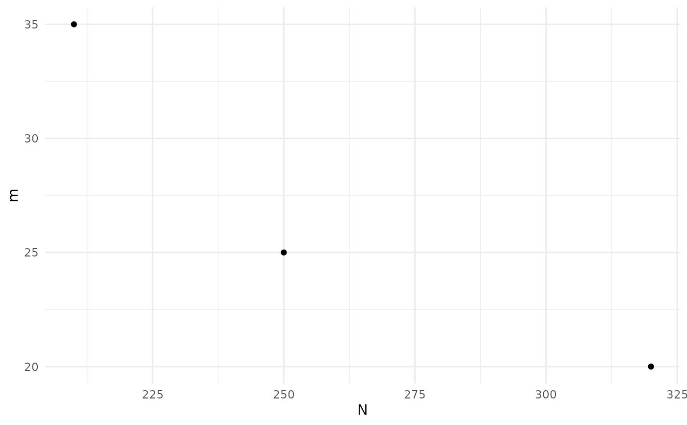

sol_init <- sol

# Take the first solution in the Pareto set and plot diagnostics:
sol$p_set[1,]
#>    m     n   N  m
#> 3 20 16.25 320 20
diag_plots(design, prob, sol)
#> [[1]]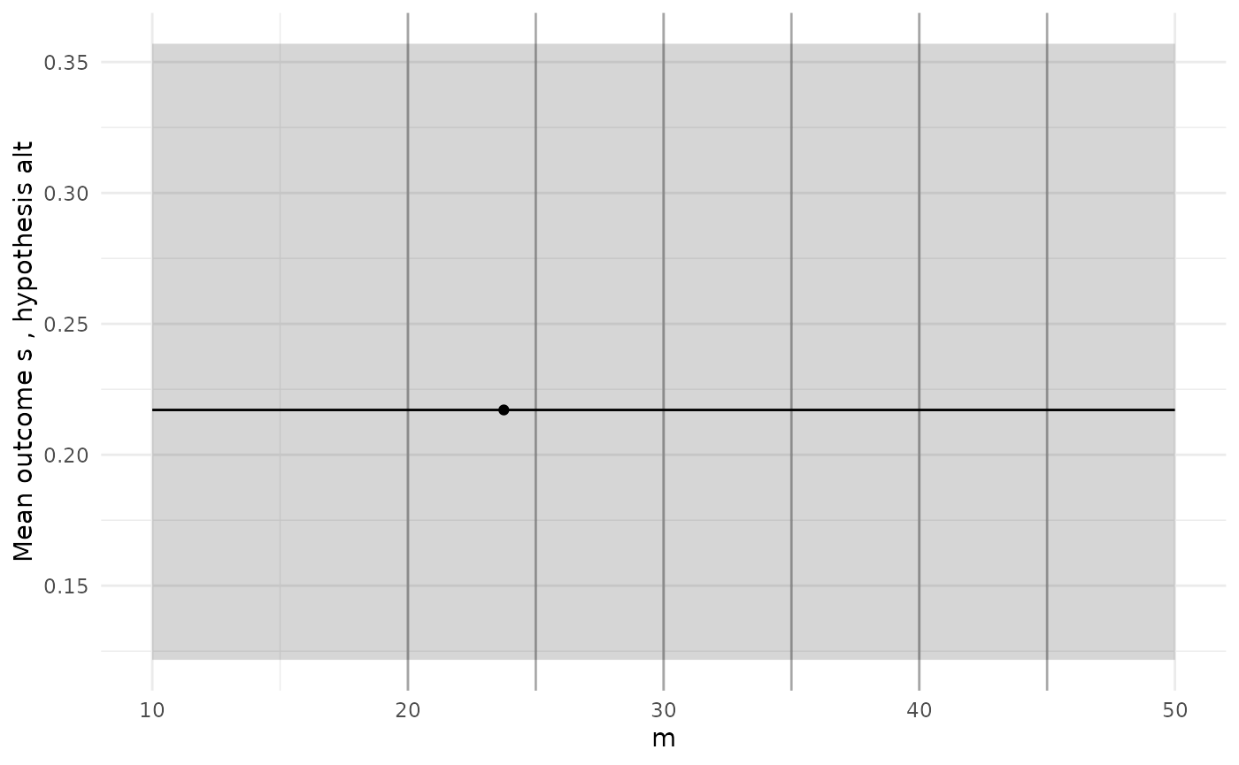

#> 
#> [[2]]

The diagnostic plots here show a GP model of the true power function which is just a constant, which we know is not true. When we see a poor initial fit like this we might want to add more simulations to designs already evaluated, or add more designs, or both. We can use the extend_initial() function for this. For example, suppose we want an extra 4 designs and for every design to have 500 simulations:

sol <- extend_initial(prob, sol, extra_points = 4, extra_N = 490)

sol$p_set[1,]
#>       m      n   N  m
#> 10 47.5 5.9375 235 47
diag_plots(design, prob, sol)
#> [[1]]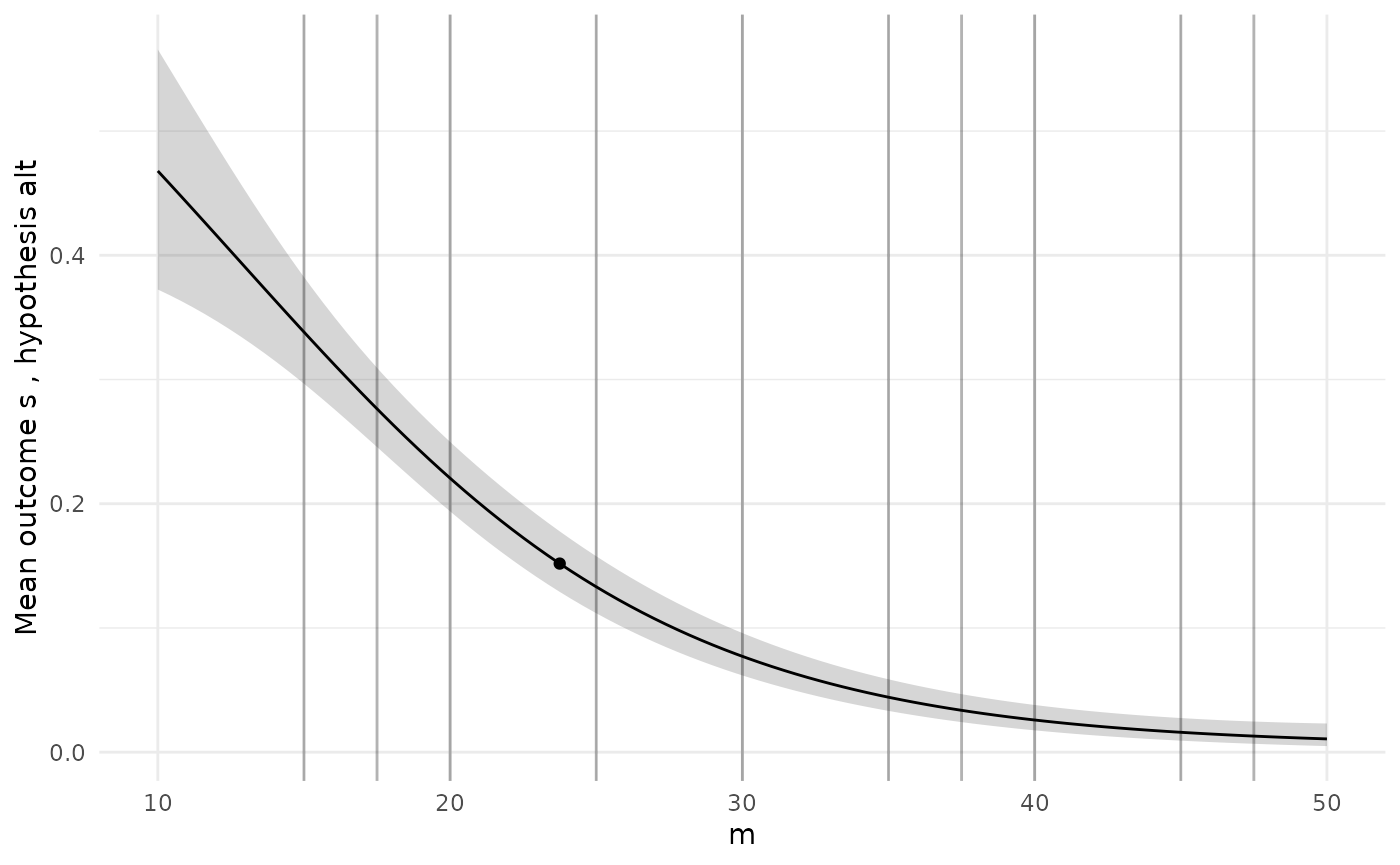

#> 
#> [[2]]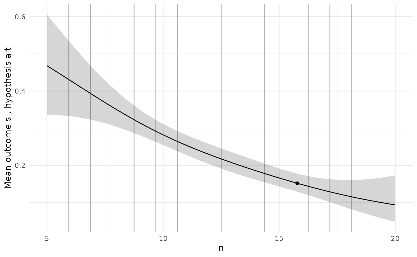

Our lots now suggest a more plausible model.